|
|
|
 |
||||
|
|
|
|
||||
| About SDSS | ||
 | ||
| The Telescopes | ||
| The Instruments | ||
| The Data | ||
| - Images | ||
| - Terms | ||
| - Spectra | ||
| - Databases | ||
| First Discoveries | ||
| Data Releases | ||
| Publications | ||
| Credits | ||
Processing the Data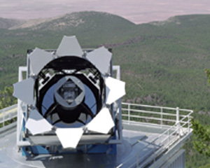
On a clear, dark night, light that has traveled through space for a billion years touches a mountaintop in southern New Mexico and enters the sophisticated instrumentation of the SDSS's 2.5-meter telescope. The light ceases to exist as photons, but the data within it lives on as digital images recorded on magnetic tape. Each image is composed of myriad pixels (picture elements); each pixel captures the brightness from each tiny point in the sky. But the sky is not made of pixels. The task of data managers for the Sloan Digital Sky Survey is to take digitized data - the pixels electronically encoded on the mountaintop in New Mexico - and turn them into real information about real things. Astronomers process the data to produce information they can use to identify and measure properties of stars and galaxies. Astronomers must be able to find, distinguish, and measure the brightness of celestial objects, and then collect the stars, galaxies, and quasars into a catalog. Computing experts describe the project as something like creating the Manhattan phone book for the heavens. Each star is like a person in the phone book, with a name and an address. There is even a Yellow Pages in the celestial directory: the spectral survey, a section containing a smaller number of entries with more detailed information. The spectral digitized data yield information about galaxies' velocities as they move away from the Earth, from which we can calculate how far away they are. Scientists must initially process the data quickly (within about a week) because SDSS astronomers need the information to configure their telescope to work most efficiently during the next dark phase of the moon. If too much time goes by, the target objects will set as the season passes. Scientists at Fermilab have led the effort to develop what the SDSS calls data-processing pipelines. A pipeline is a computer program that processes digitized data automatically to extract certain types of information. The term "pipeline" connotes the automated nature of the data processing; the data "flow" through the pipelines with little human intervention. For example, the astrometric pipeline, built by computer scientists at the U.S. Naval Observatory, determines the precise absolute two-dimensional position of stars and galaxies in the sky. In this case, digitized data from photons reaching the 2.5-meter telescope go in one end of the astrometric pipeline, and object positions come out the other. In between, along the length of the pipeline, software changes pixels into real information. The data pipelines are a collaborative effort. Princeton University scientists built the photometric pipeline, and University of Chicago scientists created the spectroscopic pipeline. Fermilab's contributions include the monitor-telescope pipeline and the pipeline that selects candidates for the spectroscopic survey. Fermilab also coordinates the smooth operation of all the pipelines. Information processing for the SDSS begins when the CCDs collect light. Charge "buckets" are converted to digitized signals and written to tape at the observatory. The tapes travel from Apache Point to Fermilab by express courier. The tapes go to Fermilab's Feynman Computing Center, where their data are read and sent into various pipelines: spectrographic data into the spectrographic pipeline, monitor telescope data into the monitor pipeline, and imaging data into the astrometric, photometric, target selection, and two other pipelines. Information about stars, galaxies and quasars comes out of the pipeline. This information is included in the Operations Database, written at Fermilab and at the Naval Observatory, which collects information needed to keep the Sky Survey running. Eventually, experimenters will pass the information in the Operations Database to the science database developed by scientists at Johns Hopkins University. The science database will make the data readily available to scientists on the project. SDSS TerminologyTo understand how data are processed, it helps to understand the terms SDSS scientists use to describe the data: A scanline is data from a single set of CCDs that sweep the same
area of sky. Each set of 5 CCDs is housed in a single dewar: each dewar has 6 sets of
CCDs separated by about 80% of the CCD width. The area of sky swept by the 6
CCD columns, or "camcols," is called a strip. A given area of sky is
imaged by performing two successive scans, offset by almost a CCD width, to
fill in a stripe.
The data stream from a single CCD in a scanline is cut into a series of
frames that measure 2048 x 1489 pixels and overlap 10% with the adjacent
frames. The frames in the 5 filters for the same part of the sky are called a field.
A run is the set of data collected from one continuous pass of the
2.5 m telescope across the sky, covering one strip. Typically, a run lasts for a few hours.
The Images
Astrometric calibrations (assigning precise coordinates to each object)
are performed by the astrometric pipeline (Astrom). The photometric calibrations
(measuring the conditions of the atmosphere during each run) are produced by the
monitor telescope pipeline (MT). Because the stars used in this
calibration are too bright to be observed by the main 2.5 m telescope,
sky patches that overlap the 2.5 m scans are observed with the Monitor
Telescope. These secondary patches are used to tie the MT photometric system to the
main 2.5 m observations.
The photometric pipeline (Photo) turns the imaging data into information about the celestial objects. Photo consists of three successive pipelines. The last of these, the Frames pipeline, operates on an individual set of five frames that cover a field. Photo corrects each frame for artifacts (bad columns, cosmic rays, etc.), corrects for detector background and sensitivity variations, finds objects in two stages (bright and faint), searches for lower surface brightness objects in a binned image, and combines the objects in the five filters. Photo then measures the objects (position, size, shape, counts), classifies them, resolves compound objects to get information about individual members, and cuts atlas images. Then, Photo writes a series of outputs: tables of measured parameters, corrected frames, sky frames four pixels square with objects subtracted, atlas images, mask frames (to cover mistakes such as saturated or interpolated pixels), and summary statistics for each frame.
To perform these calculations, the Frames pipeline needs to know the properties of the
detectors and the sky background. These properties are calculated by
the Postage Stamp Pipeline (PSP), which calculates these quantities for
the whole run and interpolates them to the center of each frame. The
PSP uses cutout images of bright (but unsaturated) stars, rejects bad
stars (double stars, etc.) and calculates the parameters of a simple point spread
function (PSF) - the shape of a stellar image. The cutouts are made
by the Serial Stamp Collecting Pipeline (SSC), which also aligns the frames
in a field. Below, we show examples of some processing steps carried out
on part of a single frame. Click on each picture for a larger image.
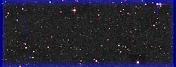
Once the imaging data have been run through these pipelines, the images from the five filters can be combined to make the beautiful color images accessible on this site. Additionally, the measured parameters of all the objects are stored in a database that astronomers can search to find objects they are interested in studying. Spectra
The purpose of the spectroscopic observations is threefold:
The spectroscopic data pipeline is designed to output these important quantities.
Like the imaging data, the spectroscopic data are processed by a large pipeline,
which takes the input CCD data and outputs completely processed spectra. The
first part of the pipeline applies corrections for detector problems and
characteristics. These corrections require a number of other pieces of data:
Furthermore, a correction is made to account for the absorption of the
Earth's atmosphere (telluric correction) and the Doppler shift due to
the Earth's motion around the sun (heliocentric correction).
Once all these corrections are applied, the pipeline extracts
individual object spectra, and then produces a one-dimensional
spectrum (flux as a function of wavelength) for each object. These
one-dimensional spectra must be wavelength calibrated, their red and blue
halves must be joined, and then the spectra be identified.
The last task, spectral identification, is important but challenging.
The spectra of galaxies can vary greatly, and spectra for stars, quasars,
and other types of objects look different. Not only do the intrinsic
properties of these objects vary, but they can be at different redshifts,
meaning we see a different portion of their spectrum. To make sense of all these
spectra, the software first tries to find all the emission lines (spectral features
due to the emission of specific wavelengths of light from atoms or
molecules) and identify them. Then, the entire spectrum is matched against
a set of templates - standard spectra of different kinds of objects - that test
how well the spectrum matches each template at different redshifts.
The best match tells us what type of object we are looking at, and
simultaneously, the object's redshift.
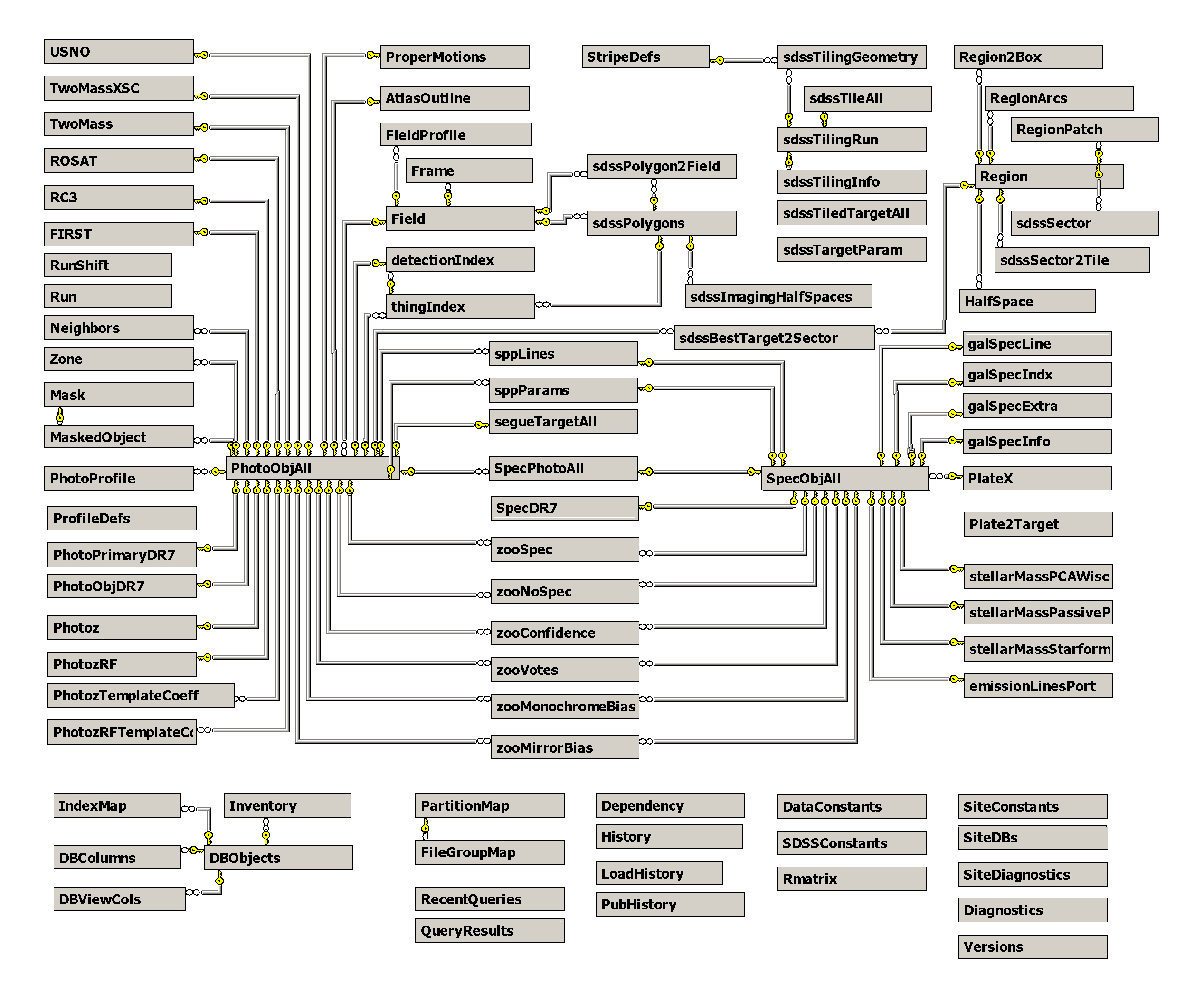
The Databases
Database Logical DesignThe processed data are stored in databases. The logical database design consists of photographic and spectrographic objects. They are organized into a pair of snowflake schemas. Subsetting views and many indices give convenient access to the conventional subsets (such as stars and galaxies). Procedures and indices are defined to make spatial lookups convenient and fast.
Since the data processing software underwent substantial changes since the survey started, we are storing two different versions of our processed images. First, we store the version of the processed data frozen at the moment when the targets for spectroscopic observations were selected. This database is called TARGDR1, where DR1 designates the version number: Data Release 1. When the data have been processed with the best available version of the software, these objects are stored in the database BESTDR1. The schema of the two databases is identical, and many of the objects appear in both, but due to the better handling of the noise, the number of objects in BESTDR1 is somewhat higher.
Database Physical DesignSkyServer initially took a simple approach to database design – and since that worked, we stopped there. The design counts on the SQL storage engine and query optimizer to make all the intelligent decisions about data layout and data access. The data tables are all created in several filegroups. The database files are spread across a single RAID0 volume. Each filegroup contains several database files that are limited to about 50Gb each. The log files and temporary database are also spread across these disks. SQL Server stripes the tables across all these files and hence across all these disks. It detects the sequential access, creates the parallel prefetch threads, and uses multiple processors to analyze the data as quickly as the disks can produce it. When reading or writing, this automatically gives the sum of the disk bandwidths (over 400 MBps peak, 180MBps typical) without any special user programming. Beyond this file group striping, SkyServer uses all the SQL Server default values. There is no special tuning. This is the hallmark of SQL Server – the system aims to have "no knobs" so that the out-of-the box performance is quite good. The SkyServer is a testimonial to that goal. Personal SkyServer
A small subset of the SkyServer database (about 1.3 GB SQL
Server database) can fit (compressed) on a CD or be
downloaded
over the web. This includes the website and all the photo and
spectrographic objects in a 6º square of the sky. This
personal SkyServer fits on laptops and desktops. It is
useful for experimenting with queries, for developing the
web site, and for giving demos. Essentially, any
classroom can have a mini-SkyServer per student. With
disk technology improvements, a large slice of the public
data will fit on a single disk by 2005.
| ||||||||||||||||||||||||||||||||

 The goal of the SDSS is to image all objects brighter than 23rd magnitude in 1/4
of the sky, roughly the area of the North Galactic Cap, in five different
wavelengths of light. Because of the way the
The goal of the SDSS is to image all objects brighter than 23rd magnitude in 1/4
of the sky, roughly the area of the North Galactic Cap, in five different
wavelengths of light. Because of the way the